Training YOLOv3 to Detect and Count Vehicles

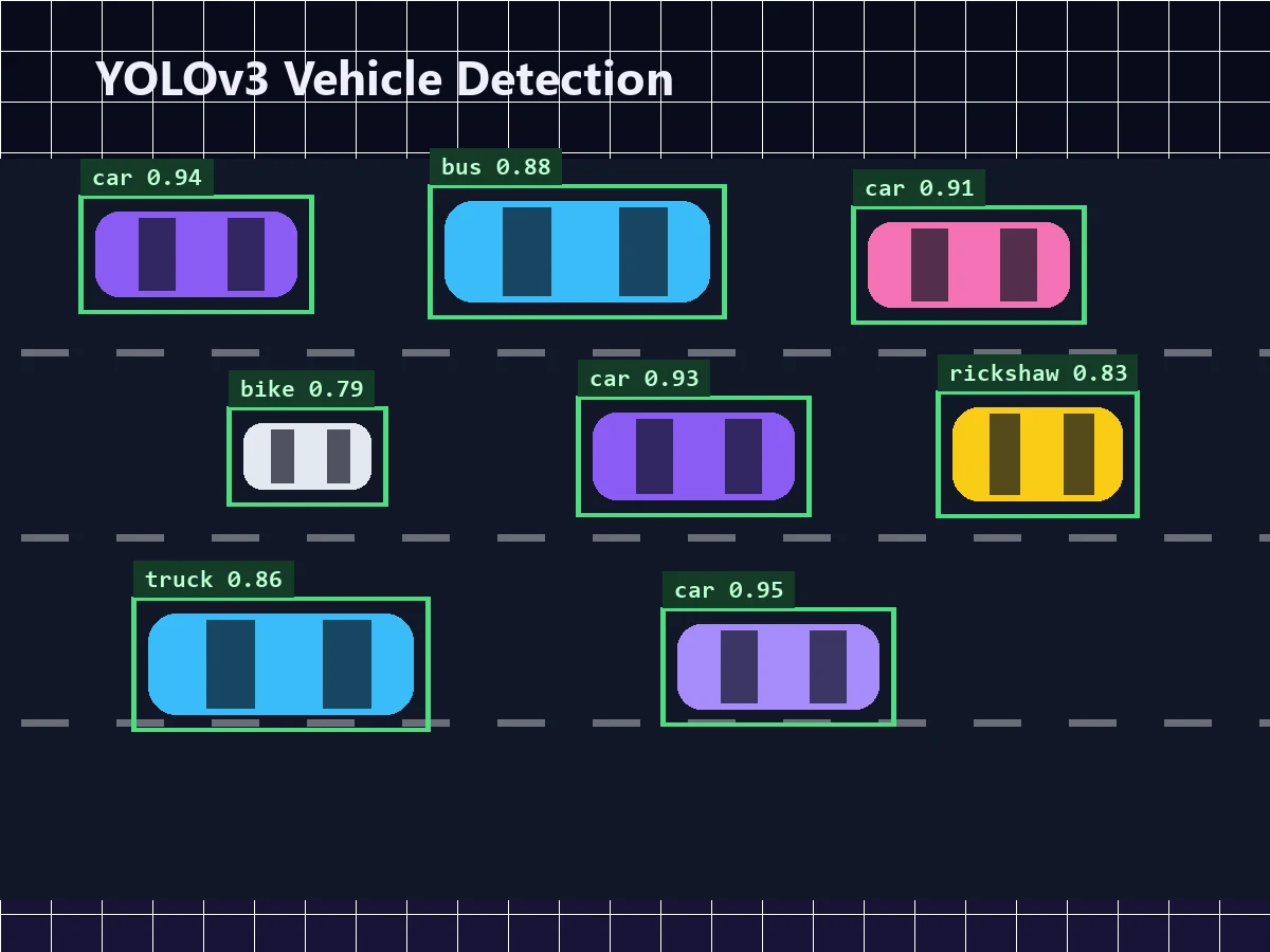
The adaptive traffic system from part one lives or dies on one question: how many vehicles of which kind are waiting at the light? Answering it in real time is a computer-vision problem, and this post covers how I solved it — training a custom YOLOv3 model to detect cars, bikes, buses/trucks, and rickshaws, running it through OpenCV, and learning the hard way that the dataset matters more than the network.

Why YOLO and not Faster R-CNN or SSD

Object detection in deep learning splits into two families. Faster R-CNN first proposes candidate regions with one network, then classifies them with another — accurate, but the two-stage pipeline costs time per frame. SSD and YOLO are single-shot: one network pass predicts bounding boxes and class labels directly, trading a little accuracy for a lot of speed.

YOLOv3 was the fit for a traffic signal because:

• It's fast enough for a deadline. The switching algorithm gives detection a five-second window (the yellow phase) to process an image and return counts. A single forward pass fits; a region-proposal pipeline gets nervous.
• It predicts at three scales, feature-pyramid style, using the Darknet-53 backbone — so it catches the bus dominating the frame and the distant motorcycle in the same pass. Traffic scenes are exactly this kind of scale chaos.
• It uses independent logistic classifiers rather than a softmax for class prediction, which is more forgiving when classes overlap visually — and "bus" vs "truck" overlap constantly, which is why they ended up sharing a class.

The dataset: where the real work was

The glamour is in the architecture; the accuracy is in the data. The training set was built by scraping vehicle images and annotating them by hand with LabelIMG, drawing bounding boxes and exporting them in YOLO's format — class id plus the box's centre, width, and height, all normalised. Around 510 images produced roughly 1,866 car, 457 motorcycle, 53 bus, and 74 truck annotations.

Those numbers teach the first lesson before training even starts: class imbalance is brutal. The model saw thirty-five cars for every bus. Combined with images collected mostly in good daylight, this set a hard ceiling on what the detector could do at night or in rain — a deep model is heavily reliant on the variety of its training conditions, not just the volume.

Configuring and training the model

Training used pre-trained weights as the starting point — transfer learning, so the network arrives already knowing edges, wheels, and windshields from millions of natural images, and only needs fine-tuning toward my four classes. Two configuration changes in the .cfg matter and are famously easy to get wrong:

# yolov3.cfg — for each [yolo] layer and the [convolutional] before it
classes = 4                      # car, bike, bus/truck, rickshaw
filters = 5 * (5 + classes)      # = 45, in the layer feeding each detection head

The filter count isn't arbitrary: each anchor predicts 4 box coordinates + 1 objectness score + one score per class, and the head needs exactly that many output channels. Set it wrong and the network either refuses to load or silently trains nonsense.

Then: train until the loss curve flattens and stays flat. No cleverness — just watching the number until it stops rewarding patience.

Inference: from image to counts

At run time, OpenCV loads the trained weights and feeds it the junction snapshot. The raw output is a flood of candidate boxes, so two filters run before anything is counted:

# Keep boxes the model is actually confident about
scores = box_confidence * box_class_probs
keep   = scores > threshold

# Collapse duplicates: many boxes, one vehicle
best = non_max_suppression(boxes, scores, iou_threshold=0.5)

Non-Max Suppression is the unsung hero of counting. The network happily draws five boxes around one car; NMS keeps the most confident box and discards every overlapping box above an IoU of 0.5. Get this wrong and your "traffic density" is really a duplicate-box density — and the signal timer inherits the lie. What survives is a JSON-like result of labels, confidences, and coordinates, which the switching algorithm parses into per-class counts.

What accuracy we actually got

Tested against videos with varying traffic, detection accuracy landed in the 75–80% range. I'll say plainly what the report says: satisfactory, not optimum — and the cause was the dataset, not the algorithm. Scraped images are cleaner, better-lit, and better-framed than real CCTV footage. The single highest-value improvement wouldn't touch the network at all: retrain on frames from the actual cameras the system would run on, with their real angles, lighting, occlusion, and grime.

That reframing — the model is a data product, not a code product — was the most valuable thing this module taught me.

Common pitfalls

1. Scraped data for a CCTV problem. Train on the distribution you'll serve. Camera height, angle, and lighting are features the model learns whether you intend it or not.
2. Ignoring class imbalance. 53 bus annotations against 1,866 cars means the model barely knows what a bus is. Oversample, augment, or gather more — but don't ignore it.
3. Wrong filter arithmetic in the config. 5 × (5 + classes) per detection head. Write the formula in a comment; future you will thank present you.
4. Trusting raw detections. Confidence thresholding and NMS aren't post-processing garnish — for a counting application they are the difference between 8 vehicles and 23.
5. Evaluating only on sunny days. Accuracy that isn't measured across lighting conditions is a best-case number wearing an average-case costume.

FAQ

Need computer vision, ML integration, or a full-stack build in Dubai, UAE? Get in touch.