Simulating City Traffic with Pygame

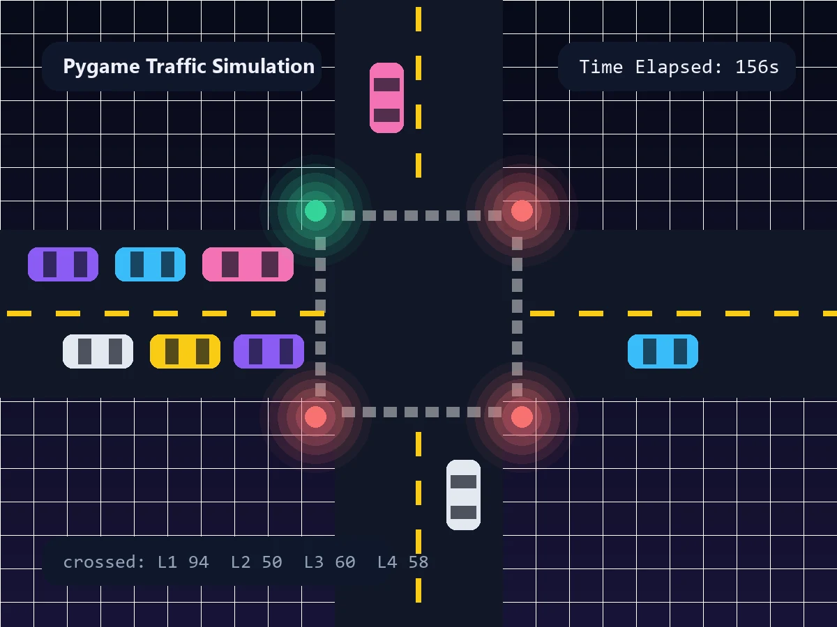
You can't A/B test a real intersection. Nobody hands a student a city junction to experiment on — and rightly so. So to prove that the adaptive system from parts one to three actually beats fixed timers, I built the test bench myself: a 4-way intersection simulator written from scratch in Pygame, with spawning traffic, working signals, and counters that don't lie. This post is about building it — and about why the simulation ended up being the most instructive module of the whole project.

Why Pygame

Pygame is a thin Python layer over the SDL library — a window, surfaces you draw on, a main loop you control, and not much else. That minimalism was the feature. A traffic simulator is fundamentally a loop that moves rectangles and enforces rules, and Pygame gives you exactly that with no framework opinions in the way: load sprites onto surfaces, blit them each frame, flip the display. Everything else — vehicles, signals, timers, physics — you own.

Building the world

The simulator came together as a stack of small, concrete steps:

• A top-view 4-way intersection image as the background.
• Top-view sprites for cars, bikes, buses, trucks, and rickshaws, resized and rotated for all four directions of travel.
• Signal images for red, yellow, and green, each with a countdown timer rendered above it and a crossed-vehicle counter beside it.
• A vehicle generator: every 0.75 seconds a new vehicle spawns with its class, direction, lane, and whether it will turn at the junction all drawn from random numbers.
• Movement rules: each class has its own speed; a vehicle keeps a gap from the one ahead, so a car stuck behind a bus slows to bus speed instead of driving through it.
• Signal rules: stop for red and yellow — unless you've already crossed the stop line when yellow hits, in which case you keep going, just like a real driver.
• Small realism touches: a dedicated bike lane to the left (common in many cities), and rightmost-lane vehicles that turn across the junction.

The distribution of traffic between directions is controllable with a cumulative array — [700, 800, 900, 1000] means 70% of vehicles spawn in lane 1 and 10% in each of the others. That one parameter is what made rigorous comparison possible.

The heart of it is the classic Pygame shape:

while time_elapsed < SIMULATION_TIME:
    handle_events()
    spawn_vehicles()          # every 0.75s, random class/lane/turn
    update_signals()          # timers, red -> green -> yellow
    move_vehicles()           # per-class speed, gap keeping, stop lines
    screen.blit(background, (0, 0))
    draw_world()              # vehicles, signals, timers, counters
    pygame.display.flip()

print_results()               # vehicles crossed per lane -> the data

Measuring instead of demoing

Here's the discipline part: the simulation wasn't a demo, it was an instrument. The metric was throughput — vehicles crossing the intersection per unit time — which is the inverse of wasted green time (a light that's green while nobody crosses). The protocol: run the adaptive system and the static system for five minutes each on identical settings — same distribution, same speeds, same turning probabilities, same gaps — across ten different traffic distributions, over an hour and a quarter of simulated traffic in total.

Sample results from the adaptive runs tell the story:

• Balanced traffic ([250,500,750,1000] — 25% per lane): 262 vehicles crossed. The static system gets close here; when every lane genuinely deserves equal time, a fixed timer is nearly right.
• Heavily skewed ([700,800,900,1000] — 70% in lane 1): 261 crossed, with 185 of them from the loaded lane. A static timer would have burned three-quarters of its green time serving trickles.
• Extreme ([940,960,980,1000] — 94% in lane 1): 211 crossed, 193 from lane 1 — the system correctly poured nearly all green time where nearly all traffic was, while the minimum-green clamp kept the other lanes alive.

Averaged across all runs, the adaptive system moved about 23% more vehicles than fixed timers — and the gain grew with skew, which matters because skewed is what real traffic looks like.

What building a simulator teaches you

More than any other module, this one changed how I work. Three lessons that came home:

1. If you can't measure it, you built a demo. The counters, the elapsed clock, the printed lane-wise results — the boring instrumentation is what turned "look, it works" into a defensible 23%.
2. Fairness in comparison is everything. The two systems ran with identical spawn seeds of conditions — distributions, speeds, gaps, turning odds. Change two variables at once and your improvement number means nothing.
3. Realism is a budget, spend it where it changes the answer. Gap-keeping and stop-line behaviour affect throughput, so they were worth building. Pretty car sprites don't, but they cost almost nothing and made the demo legible to non-engineers — which a thesis defence also needs.

That's the same mindset I bring to load-testing an e-commerce checkout or benchmarking a queue worker today: build the instrument first, hold everything constant but one variable, then believe the number.

Common pitfalls

1. Comparing systems under different traffic. Identical conditions or the comparison is fiction.
2. Spawning vehicles uniformly and calling it realistic. Real junctions are skewed; a simulator that can't express skew can't test the very case adaptive signals exist for.
3. Forgetting driver behaviour at yellow. Vehicles past the stop line must continue; stopping them mid-junction deadlocks the model and never happens on a real road.
4. Ignoring vehicle interaction. Without gap-keeping, a bus and the cars behind it discharge at fantasy speeds and flatter your throughput numbers.
5. Running once and reporting it. One five-minute run is an anecdote. Ten distributions, repeated, is data.

FAQ

From simulations to production systems — if you need an engineer who measures before claiming, get in touch.